Vector Fields

Definition

A vector field is a function which assigns each point in an $n$-dimensional space a corresponding vector of $m$ dimensions. Vector fields are commonly depicted, in 2D space for example, as a 2D graph in which every point $(x,y)$ serves as the starting point for a 2D vector, $\vec{F}(x,y)$. In 3D space, ${\mathbb{R}}^3$, each point is assigned a 3D vector, $\vec{F}(x,y,z)$. A vector field is defined as a function of the coordinates that make up its domain space, for example, a 3D vector field will be a function of $x$, $y$, and $z$, or of $i$, $j$, and $k$. Therefore,

$$\vec{F}(x,y,z)=\left(\begin{array}{c}{F}_1(x,y,z)\\ F_2(x,y,z)\\ F_3(x,y,z)\end{array}\right)=F_1(x,y,z)\hat{x}+F_2(x,y,z)\hat{y}+F_3(x,y,z)\hat{z}$$

where $\hat{x}$, $\hat{y}$, and $\hat{z}$ are orthogonal unit vectors that define a 3D space. An example vector field in 2 dimensions might be,

$$\vec{F}(x,y)=\left(\begin{array}{c}-y\\ x\end{array}\right)=-y\hat{x}+x\hat{y}$$

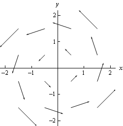
and would be visualized as, One can see here that at each point $(x,y)$, there is a vector equal to $\left(\begin{array}{c}-y\\ x\end{array}\right)$. At $(1,2)$, we see a vector equal to $\left(\begin{array}{c}-2\\ 1\end{array}\right)$.

A sample 3D vector field might be,

$$\vec{F}(x,y,z)=\left(\begin{array}{c}2x\\ -2y\\ -2x\end{array}\right)=2x\hat{x}-2y\hat{y}-2x\hat{z}$$

which is visualized as,

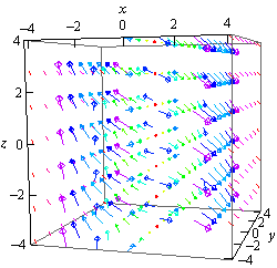
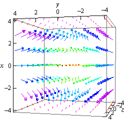
We can see here, too, that at a point $(1,2,3)$ there is a vector equal to $\left(\begin{array}{c}2\\ -4\\ -2\end{array}\right)$. For much of calculus and physics, a vector field is required to be (and naturally is) smooth at all points.

The ‘Del’ Operator

We must define a symbolic vector, one which has not real dimensions but which must be a vector for us to use it in vector math, which we will refer to as ‘del’ and which we will denote $\vec{\nabla }$. This symbolic vector will have components $\vec{\nabla }=⟨\frac{\partial }{\partial x},\frac{\partial }{\partial y},\frac{\partial }{\partial z}⟩$, which may be applied to a scalar function, $F(x,y,z)$, or to a vector function, $\vec{F}(x,y,z)=⟨F_1(x,y,z),F_2(x,y,z),F_3(x,y,z)⟩$.

We can apply the del operator to the scalar function $F$ as follows,

$$\vec{\nabla }F=⟨\frac{\partial F}{\partial x},\frac{\partial F}{\partial y},\frac{\partial F}{\partial z}⟩$$

This is called the gradient of $F$, written $grad\vec{F}=\vec{\nabla }F$, and is a vector.

We can apply the del operator to the vector function $\vec{F}$ in two ways, in a dot product or in a cross product, as follows,

$$\vec{\nabla }\cdot \vec{F}=\frac{\partial F_1}{\partial x}+\frac{\partial F_2}{\partial y}+\frac{\partial F_3}{\partial z}$$

which is called the divergence of $\vec{F}$, written $div\vec{F}=\vec{\nabla }\cdot \vec{F}$, and is a scalar; or,

$$\vec{\nabla }\times \vec{F}=\left|\begin{array}{c}\hat{x}\hat{y}\hat{z}\\ \frac{\partial }{\partial x}\frac{\partial }{\partial y}\frac{\partial }{\partial z}\\ F_1{F}_2{F}_3\end{array}\right|=(\frac{\partial F_3}{\partial y}-\frac{\partial F_2}{\partial z})\hat{x}+(\frac{\partial F_1}{\partial z}-\frac{\partial F_3}{\partial x})\hat{y}+(\frac{\partial F_2}{\partial x}-\frac{\partial F_1}{\partial y})\hat{z}$$

which is called the curl of $\vec{F}$, written $curl\vec{F}=\vec{\nabla }\times \vec{F}$, and is a vector.

There is a second way to apply the del operator to a scalar function which is commonly used,

$$\vec{\nabla }\cdot \vec{\nabla }F=\frac{{\partial }^2{F}_1}{{\partial x}^2}+\frac{{\partial }^2{F}_2}{{\partial y}^2}+\frac{{\partial }^2{F}_3}{{\partial z}^2}=\Delta F$$

which is called the Laplacian of $F$. Laplace’s differential equation is $\Delta F=\vec{\nabla }\cdot \vec{\nabla }F=0$, and any solution to this which is class $C^2$ is a harmonic function. It should be obvious that this operation is simply taking the divergence of the gradient field of $F$.

Gradient Fields

Divergence

Curl

Curl is a measure of how much a vector field rotates at a given point. We calculate curl as the cross product $\vec{\nabla }\times \vec{F}$, which results in another vector field function that represents curl values,

$$\begin{gathered} curl\vec{F}=\vec{\nabla }\times \vec{F}=\left|\begin{array}{c}\hat{i}\hat{j}\hat{k}\\ \frac{\partial }{\partial x}\frac{\partial }{\partial y}\frac{\partial }{\partial z}\\ PQR\end{array}\right| \\ =(\frac{\partial R}{\partial y}-\frac{\partial Q}{\partial z})\hat{i}+(\frac{\partial P}{\partial z}-\frac{\partial R}{\partial x})\hat{j}+(\frac{\partial Q}{\partial x}-\frac{\partial P}{\partial y})\hat{k} \end{gathered}$$

But let us first understand the concept of curl from first principles.

Curl in 1-Dimension

If we have a vector field in one dimension, it has no curl: space consists only of a single line, and every point $(x)$ along the single dimension is assigned a vector represented as $⟨x⟩$, which has magnitude as well as a direction of either forward or backward, $+$ or $-$.

Curl in 2-Dimensions

If we have a vector field that exists in two dimensions, then each point $(x,y)$ is assigned a vector $\vec{f}(x,y)=⟨f_1(x,y),f_2(x,y)⟩$, and any $\vec{f}$ can curl in either a clockwise or counter clockwise direction. That is, compared to the vectors immediately adjacent to it, a vector at a single point $\vec{f}(x,y)$ can have either a larger or smaller $x$-component (indicating rotation about the y-axis), and/or a larger or smaller $y$-component (indicating rotation about the x-axis).

Differential Derivation

For a vector $\vec{f}$, $f_1$ is the $x$-component and $f_2$ is the $y$-component. We can conceive of these components as a left-to-right force and an up-and-down force that act on the final vector, and if we sweep a single point through space, it will experience many different lateral or vertical forces according to the function $\vec{f}$. If we sweep a point along a horizontal line parallel to the x-axis, then an upward vertical force, a positive $f_2$, will represent a counterclockwise rotation about the centerpoint; a downward force, a negative $f_2$, will represent a clockwise rotation. Therefore, to discover the curl of $\vec{f}$ along a horizontal line, we must take the derivative of $f_2$ with respect to $x$, $\frac{\partial f_2}{\partial x}$.

For the same reason, by sweeping a point along a vertical line and observing the value of $f_1$ at each position, the curl of $\vec{f}$ along a vertical line will be the derivative of $f_1$ with respect to $y$, $\frac{\partial f_1}{\partial y}$.

Then, to find the total curl of $\vec{f}$, we must consider both $\frac{\partial f_2}{\partial x}$ and $\frac{\partial f_1}{\partial y}$. How do we relate them?

Let’s return to basic concepts. At the point $(x,y)$, the vector field is $\vec{f}(x,y)=⟨f_1(x,y),f_2(x,y)⟩$. Then at an infinitesimal distance away from that point, at $(x+\Delta x,y)$, the vector field is

$$\vec{f}(x+\Delta x,y)\approx ⟨f_1(x,y)+\frac{\partial f_1(x,y)}{\partial x}\Delta x,f_2(x,y)+\frac{\partial f_2(x,y)}{\partial x}\Delta x⟩$$

and at a point $(x,y+\Delta y)$,

$$\vec{f}(x,y+\Delta y)\approx ⟨f_1(x,y)+\frac{\partial f_1(x,y)}{\partial y}\Delta y,f_2(x,y)+\frac{\partial f_2(x,y)}{\partial y}\Delta y⟩$$

Then these changes can be represented as a matrix:

$$\left[\begin{array}{c}{f}_1(x,y)\\ f_2(x,y)\end{array}\right]=\left[\begin{array}{c}\frac{\partial f_1}{\partial x}\frac{\partial f_1}{\partial y}\\ \frac{\partial f_2}{\partial x}\frac{\partial f_2}{\partial y}\end{array}\right]\left[\begin{array}{c}\Delta x\\ \Delta y\end{array}\right]$$

This 2x2 matrix is a Jacobian. Any matrix can be broken apart into a symmetric and antisymmetric component: $M=S+A=\frac{1}{2}(M+M^T)+\frac{1}{2}(M-M^T)$. Therefore this Jacobian’s antisymmetric component is,

$$A=\frac{1}{2}\left[\begin{array}{c}0\frac{\partial f_1}{\partial y}-\frac{\partial f_2}{\partial x}\\ \frac{\partial f_2}{\partial x}-\frac{\partial f_1}{\partial y}0\end{array}\right]=\frac{1}{2}\left[\begin{array}{c}0-(\frac{\partial f_2}{\partial x}-\frac{\partial f_1}{\partial y})\\ \frac{\partial f_2}{\partial x}-\frac{\partial f_1}{\partial y}0\end{array}\right]$$

We now have a relationship between $\frac{\partial f_2}{\partial x}$ and $\frac{\partial f_1}{\partial y}$. This matrix $A$ represents an infinitesimal rotation, and the off-diagonal element represents the curl of $\vec{f}$. Thus we have,

$$curl\vec{f}=\frac{\partial f_2(x,y)}{\partial x}-\frac{\partial f_1(x,y)}{\partial y}=\left|\begin{array}{c}\frac{\partial }{\partial x}\frac{\partial }{\partial y}\\ f_1(x,y)f_2(x,y)\end{array}\right|=\vec{\nabla }\times \vec{f}$$

Integral Derivation

Suppose the 2D vector field $\vec{f}$ has some closed curve within it, $C$, which itself encloses a 2D space $A$, and that $C$ can be parameterized by a function $\vec{r}(t)$. Then, for every infinitesimal section of $\vec{r}$, $d\vec{r}$, we can compute the dot product of that small vector with the vector of $\vec{f}$ at that same point, to find the “circulation” of $\vec{f}$ along $C$, which is really just a measure of how much the vector field aligns with a tangent vector to $C$ at every point along $C$. Thus we have the integral along a closed curve of $\vec{f}$ dot-producted with an infinitesimal section of $\vec{r}$:

$$circ\vec{f}={\oint }_C\vec{f}\cdot d\vec{r}$$

We can see that, according to this formulation, a longer curve $C$ will result in a larger circulation, which is improper: our goal is to measure the circulation of the vector field without considerations of $C$ or $A$. For that reason we will also normalize the area to find the circulation per unit area:

$$circ\vec{f}=\frac{1}{|A|}{\oint }_C\vec{f}\cdot d\vec{r}$$

where $|A|$ is the area of $A$. This integral can be used to find the curl of $\vec{f}$ at a single point if we shrink the radius (or area, if not a circle) of $A$ down to $0$ while keeping it centered at $(x,y)$, as here:

$$curl\vec{f}=\underset{|A|\to 0}{\lim }\frac{1}{|A|}{\oint }_C\vec{f}\cdot d\vec{r}$$

Instead of conceiving of curl as instantaneous rotation in one direction or the other, we are now thinking of it as the total rotation-per-unit-area of an infinitesimally small area. Greene’s Theorem states,

$${\oint }_C\vec{F}\cdot d\vec{r}={\iint }_A(\vec{\nabla }\times \vec{F})da$$

Here we can see that this former expression of curl is identical to the differential form.

The Laplacian

Example

Let $F(x,y,z)=x^2-y^2+2yz$. Then,

$$\begin{gathered} gradF=\vec{\nabla }F=⟨2x,-2y+2z,2y⟩ \\ \Delta F=\vec{\nabla }\cdot \vec{\nabla }F=2-2=0 \end{gathered}$$

Therefore $F$ is harmonic.