The Taylor Series

The Taylor Series is a Power Series which is used to represent any function as an infinite sum of polynomials, which is useful for representing difficult functions in a form that is easier to work with.

Definition

$$f(x)=\sum _{n=0}^{\infty }\frac{f^{(n)}(a)}{n!}(x-a{)}^n\text{\hspace{1em}(1)}$$

Derivation

The equation for the Taylor Series is formidable to beginners, even though its mechanics can be quickly deduced. One should wonder what each part does, and why it is necessary to approximate a function. I will offer a chain of derivation that was satisfactory to me, in the hopes that others see the clear line of derivation as I do.

The goal of the Taylor Series is to approximate a function about a point by using an infinite power series. In truth, the Taylor Series is only possible due to the fact that an infinite series of polynomials, if modified by the proper series of coefficients, can take the shape of any function.

Why Polynomials?

To represent an arbitrary function, we require a “building block” which can take any shape at any point. Polynomials have definite shapes at all points: $y=x^2$ is clearly an upward-facing “U” shape, $y=x^3$ is a sideways “S” shape, etc., so how can polynomials be a suitable class of functions to represent any shape?

Take this illustration: on the interval $[-1,1]$, we plot the polynomials $x$, $x^2$, $x^3$, $x^4$, and $x^5$, each multiplied by the coefficient defined in the Taylor Series, in this case being $1$, $\frac{1}{2}$, $\frac{1}{6}$, $\frac{1}{24}$, and $\frac{1}{120}$ respectively.

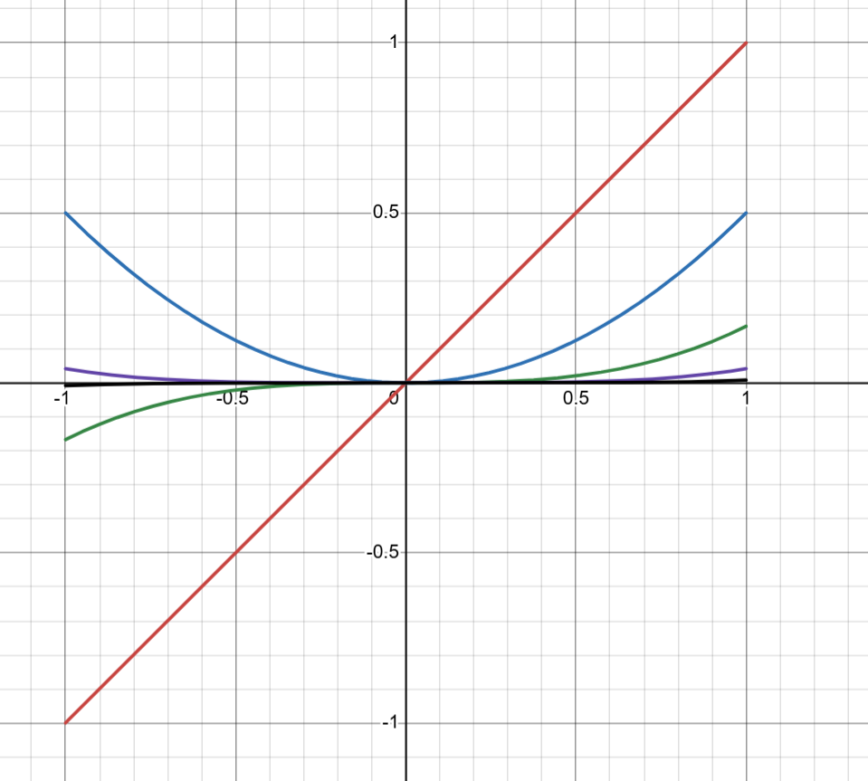
We see clearly here that $y=x$ is dominant on this interval: it has a greater magnitude than the other functions at all points, $x>x^2>x^3>x^4>x^5$ on $[-1,1]$. If we wanted to represent an arbitrary function within this interval, we must first manage the coefficient governing $y=x$ before considering any other powers of $x$ or their coefficients. Higher orders of $x$, such as $x^2$ or $x^5$, are less important here. However, let me now shift the interval from $[-1,1]$ to $[-1,5]$, so we can see if this behavior holds for values beyond $x=1$.

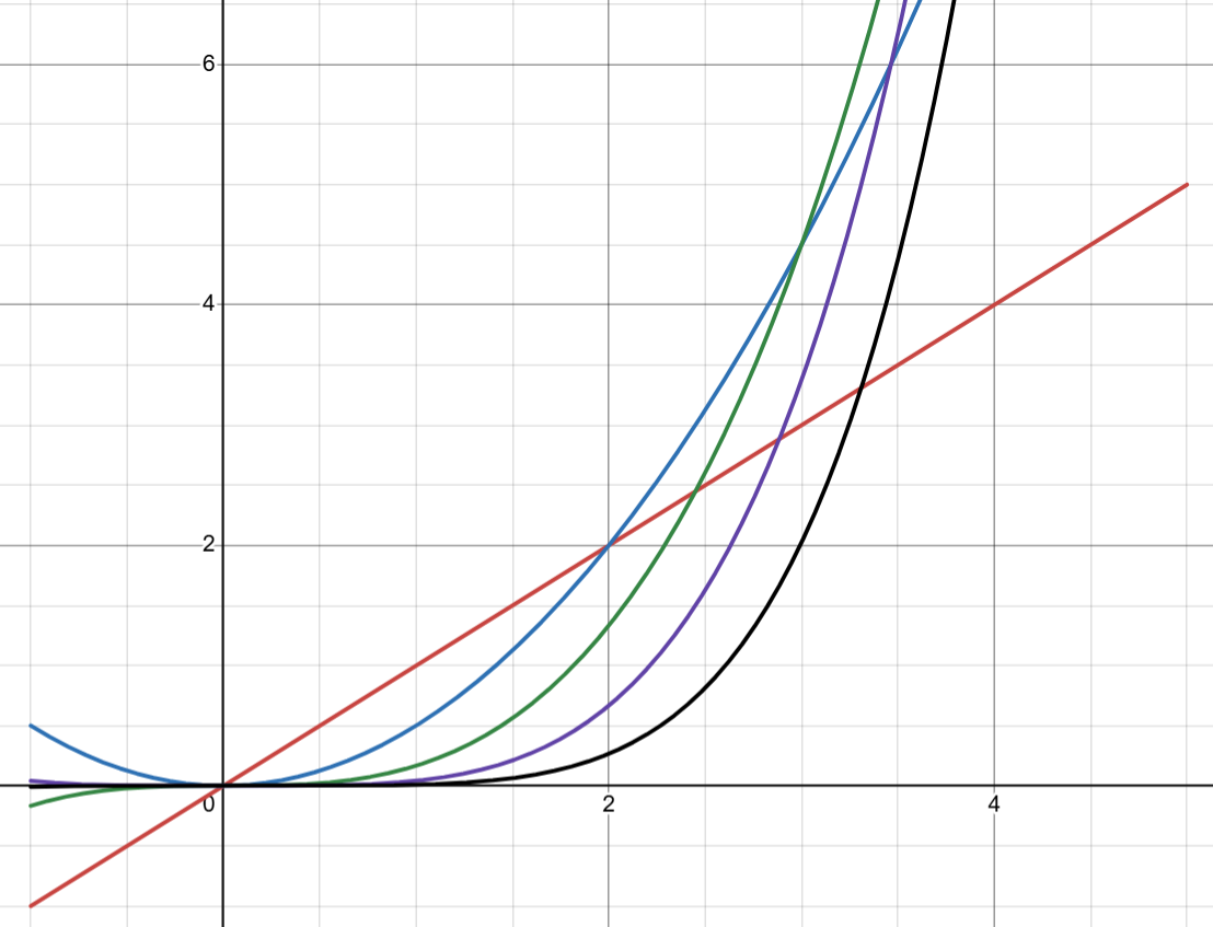
Now we see an interesting property emerge! $y=x$ remains dominant while $x<2$, but once $x$ becomes greater than 2 it is actually $y=x^2$ that becomes the dominant function, and it remains dominant until $x=3$, after which it is overtaken by $y=x^3$. Then $y=x^3$ is dominant before being overtaken by $y=x^4$, and so on. Thus it is revealed that the dominance of $y=x$ is restricted to a finite window, $[-2,2]$; and likewise there is an interval on which $y=x^2$ is dominant above all other functions, including those of higher order than itself, that being $[2,3]$ as well as $[-3,-2]$ . An infinite comparison of powers of $x$ would reveal that each power has a specific window in which it takes precedence before being overpowered by the next in line. It is also revealed that these windows are dependent on distance from the “centerpoint” being considered ($x=0$ in this example).

Therefore to fulfill the task of representing any arbitrary function, an infinite series of polynomials is apparently a highly qualified candidate (polynomials are perhaps uniquely suited for this challenge), but only if they are modified by an infinite series of coefficients which “press down” on the higher-order functions before they can “take off” and overtake the lower order functions. Without these coefficients, a normal comparison of $y=x$ through $y=x^5$ would show that for $x>1$ it is $x^5$ that is dominant at all points, thus ruining this elegant emergent quality. It is also appropriate that the higher-order powers of $x^n$ are “clamped down” in proportion to the power to which $x$ is raised, beautifully encapsulated in the Taylor coefficient’s divisor being $n!$.

We see these windows clearly in a graphic like this, below. For each higher power of $x$ that is added to the sum, the resulting function approximates the desired function better only at a certain distance from the centerpoint! It is visually evident that using this method, we are able to “steer” the function upwards or downwards as we move away from the centerpoint with almost total control, and without affecting the parts of the resulting function that we’ve “moved past”.

For these reasons, and without knowing precisely what the desired coefficients are (I willfully jumped the gun earlier to demonstrate the validity of this idea), we can say that there is an infinite series of polynomials which can approximate any arbitrary function, which conforms to the following formulae:

$$f(x)=\sum _{n=0}^{\infty }{c}_n(x-a{)}^n\text{\hspace{1em}(2)}$$

where $a$ represents the centerpoint being considered along the x-axis, and $c_n$ is the series of coefficients.

An astute mathematician will also note that this property of polynomials to approximate a function only holds if the desired function is continuous. A discontinuity can never be bridged by smooth polynomials.

Coefficients

We have seen why polynomials are suitable as “building blocks” for the Taylor Series, and that they only qualify if each term is modified by a coefficient that is finely tuned to the specific function we want to approximate. Therefore out next challenge is discovering how to acquire the right series of coefficients.

We can begin by performing a common mathematical trick, that of presuming that there does exist a proper series of coefficients, and then working backwards to discover what that series might be. So any function we might want to approximate could be described as follows:

$$f(x)=c_0+c_1(x-a)+c_2(x-a{)}^2+c_3(x-a{)}^3+\dots \text{\hspace{1em}(3)}$$

This is the Taylor Series (2) expanded. Now it is also possible to plug $a$, our centerpoint, into this function,

$$f(a)=c_0+c_1\ast 0+c_2\ast 0+c_3\ast 0+\dots$$

therefore $c_0=f(a)$. We can also differentiate (3) to obtain the following, and then plug in $a$ once more:

$$\begin{gathered} f^{\prime }(x)=c_1+2c_2(x-a)+3c_3(x-a{)}^2+\dots \\ {f}^{\prime }(a)=c_1+2c_2\ast 0+3c_3\ast 0+\cdots =c_1 \end{gathered}$$

Therefore $c_1=f^{\prime }(a)$. We can differentiate once more and plug in $a$ again:

$$\begin{gathered} f^{\prime \prime }(x)=2c_2+6c_3(x-a)+12c_4(x-a{)}^2+\dots \\ {f}^{\prime \prime }(a)=2c_2+6c_3\ast 0+12c_4\ast 0+\cdots =2c_2 \end{gathered}$$

to find that $2c_2=f^{\prime \prime }(a)$ or $c_2=\frac{f^{\prime \prime }(a)}{2}$. One can now see that any $c_n$ will be equal to the n-th derivative of $f(a)$, divided by the factorial of however many times the function has been differentiated. It is significant that for any order of differentiation, all lower powers are removed and all higher powers go to zero. Finding the value of $c_{11}$ will have one differentiating the function 11 times, which will eliminate the first 10 terms, $c_1-c_{10}$, which will lead to a divisor of $1\ast 2\ast 3\ast 4\ast 5\ast 6\ast 7\ast 8\ast 9\ast 10\ast 11=11!$ and thence to $c_{11}=\frac{f^{11}(a)}{11!}$.

Following this pattern, we can establish the factor, $c_n$, which modifies each term of the Taylor Series, as the following:

$$c_n=\frac{f^n(a)}{n!}$$

An astute mathematician will notice that this coefficient is only possible for functions which are infinitely differentiable, and which remain continuous for each differentiation (this is because we assumed that each differentiation can also be represented by an infinite series with coefficients, and that is only possible if the differentiation is also continuous).

The Interval

We have spoken above about the restrictions of approximating a function, one of which is that the approximation cannot begin at all points at once. We must select a starting point, and then if possible, the approximation can extend to infinity, but we must first select a point at which to begin. This point has been the “centerpoint”, $x=a$, on the open interval, $(j,k)$, for which the function satisfies the requirements of the Taylor Series (see below in The Finished Equation).

If a function cannot be represented by a Taylor Series on some interval due to a discontinuity, for example, it may still be possible on another interval. This can be seen with the absolute value of $x$, $y=|x|$, which is neither differentiable nor smooth at $x=0$, therefore a Taylor Series for the whole function is impossible. However, on the interval (15, 48), the function is equal to $y=x$ and the Taylor Series is absolutely possible.

Also, due to the differentiability requirement of the Series, the interval must be open, not closed.

The Finished Equation

Thus we have derived both parts of the Taylor Series, the coefficient and the polynomial, and hopefully I have explained their derivation to a satisfactory extent. Our finished Series equation is,

$$f(x)=\sum _{n=0}^{\infty }\frac{f^{(n)}(a)}{n!}(x-a{)}^n\text{\hspace{1em}(1)}$$

This series is able to represent any function as a sum of polynomials, allowing us to perform many operations on a function which would otherwise seem impossible or confusing. We also have a list of requirements that a function must meet in order for a Taylor Series to be possible:

• The function is continuous on the interval, and all derivatives of the function are continuous on the interval. Mathematically, we say $f\in C^{\infty }(j,k)$.
• The function is differentiable on the interval.
• When the function is differentiated, it still

Convergence

Take the function $f(x)=\frac{1}{1-x}$. This function is undefined at $x=1$: from the left, it goes to $\infty$, and from the right it goes to $-\infty$, with a discontinuity at $x=1$. Therefore, any series approximation performed about a point to the left of this discontinuity will converge to $f(x)<1$, while if performed about a point to the right of it, it will approximate $f(x)>1$.

Radius of Convergence

Examples